Installing JAGS
In addition to installing the jagsUI package, we also
need to separately install the free JAGS software, which you can
download here.
Once that’s installed, load the jagsUI library:
Typical jagsUI Workflow
- Organize data into a named
list - Write model file in the BUGS language
- Specify initial MCMC values (optional)
- Specify which parameters to save posteriors for
- Specify MCMC settings
- Run JAGS
- Examine output
1. Organize data
We’ll use the longley dataset to conduct a simple linear
regression. The dataset is built into R.
data(longley)
head(longley)
#      GNP.deflator     GNP Unemployed Armed.Forces Population Year Employed
# 1947         83.0 234.289      235.6        159.0    107.608 1947   60.323
# 1948         88.5 259.426      232.5        145.6    108.632 1948   61.122
# 1949         88.2 258.054      368.2        161.6    109.773 1949   60.171
# 1950         89.5 284.599      335.1        165.0    110.929 1950   61.187
# 1951         96.2 328.975      209.9        309.9    112.075 1951   63.221
# 1952         98.1 346.999      193.2        359.4    113.270 1952   63.639
We will model the number of people employed (Employed)
as a function of Gross National Product (GNP). Each column
of data is saved into a separate element of our data list. Finally, we
add a list element for the number of data points n. In
general, elements in the data list must be numeric, and structured as
arrays, matrices, or scalars.
2. Write BUGS model file
Next we’ll describe our model in the BUGS language. See the JAGS manual for detailed information on writing models for JAGS. Note that data you reference in the BUGS model must exactly match the names of the list we just created. There are various ways to save the model file, we’ll save it as a temporary file.
# Create a temporary file
modfile <- tempfile()

#Write model to file
writeLines("
model{

  # Likelihood
  for (i in 1:n){
    # Model data
    employed[i] ~ dnorm(mu[i], tau)
    # Calculate linear predictor
    mu[i] <- alpha + beta*gnp[i]
  }

  # Priors
  alpha ~ dnorm(0, 0.00001)
  beta ~ dnorm(0, 0.00001)
  sigma ~ dunif(0,1000)
  tau <- pow(sigma,-2)

}
", con=modfile)
3. Initial values
Initial values can be specified as a list of lists, with one list
element per MCMC chain. Each list element should itself be a named list
corresponding to the values we want each parameter initialized at. We
don’t necessarily need to explicitly initialize every parameter. We can
also just set inits = NULL to allow JAGS to do the
initialization automatically, but this will not work for some complex
models. We can also provide a function which generates a list of initial
values, which jagsUI will execute for each MCMC chain. This
is what we’ll do below.
4. Parameters to monitor
Next, we choose which parameters from the model file we want to save
posterior distributions for. We’ll save the parameters for the intercept
(alpha), slope (beta), and residual standard
deviation (sigma).
params <- c('alpha','beta','sigma')5. MCMC settings
We’ll run 3 MCMC chains (n.chains = 3).
JAGS will start each chain by running adaptive iterations, which are
used to tune and optimize MCMC performance. We will manually specify the
number of adaptive iterations (n.adapt = 100). You can also
try n.adapt = NULL, which will keep running adaptation
iterations until JAGS reports adaptation is sufficient. In general you
do not want to skip adaptation.
Next we need to specify how many regular iterations to run in each
chain in total. We’ll set this to 1000 (n.iter = 1000).
We’ll specify the number of burn-in iterations at 500
(n.burnin = 500). Burn-in iterations are discarded, so here
we’ll end up with 500 iterations per chain (1000 total - 500 burn-in).
We can also set the thinning rate: with n.thin = 2 we’ll
keep only every 2nd iteration. Thus in total we will have 250 iterations
saved per chain ((1000 - 500) / 2).
The optimal MCMC settings will depend on your specific dataset and model.
6. Run JAGS
We’re finally ready to run JAGS, via the jags function.
We provide our data to the data argument, initial values
function to inits, our vector of saved parameters to
parameters.to.save, and our model file path to
model.file. After that we specify the MCMC settings
described above.
out <- jags(data = jags_data,
            inits = inits,
            parameters.to.save = params,
            model.file = modfile,
            n.chains = 3,
            n.adapt = 100,
            n.iter = 1000,
            n.burnin = 500,
            n.thin = 2)
#
# Processing function input.......
#
# Done.
#
# Compiling model graph
#    Resolving undeclared variables
#    Allocating nodes
# Graph information:
#    Observed stochastic nodes: 16
#    Unobserved stochastic nodes: 3
#    Total graph size: 74
#
# Initializing model
#
# Adaptive phase, 100 iterations x 3 chains
# If no progress bar appears JAGS has decided not to adapt
#
#
#  Burn-in phase, 500 iterations x 3 chains
#
#
# Sampling from joint posterior, 500 iterations x 3 chains
#
#
# Calculating statistics.......
#
# Done.
We should see information and progress bars in the console.
If we have a long-running model and a powerful computer, we can tell
jagsUI to run each chain on a separate core in parallel by
setting argument parallel = TRUE:
out <- jags(data = jags_data,
            inits = inits,
            parameters.to.save = params,
            model.file = modfile,
            n.chains = 3,
            n.adapt = 100,
            n.iter = 1000,
            n.burnin = 500,
            n.thin = 2,
            parallel = TRUE)
While this is usually faster, we won’t be able to see progress bars when JAGS runs in parallel.
7. Examine output
Our first step is to look at the output object out:
out
# JAGS output for model '/tmp/Rtmp32mRJh/fileab4a797205d3', generated by jagsUI.
# Estimates based on 3 chains of 1000 iterations,
# adaptation = 100 iterations (sufficient),
# burn-in = 500 iterations and thin rate = 2,
# yielding 750 total samples from the joint posterior.
# MCMC ran for 0.001 minutes at time 2026-01-29 15:20:58.879265.
#
#            mean    sd   2.5%    50%  97.5% overlap0 f  Rhat n.eff
# alpha    51.845 0.797 50.250 51.819 53.444    FALSE 1 1.005   465
# beta      0.035 0.002  0.031  0.035  0.038    FALSE 1 1.005   471
# sigma     0.729 0.145  0.508  0.707  1.067    FALSE 1 1.000   750
# deviance 33.487 2.871 30.032 32.781 40.779    FALSE 1 1.002   750
#
# Successful convergence based on Rhat values (all < 1.1).
# Rhat is the potential scale reduction factor (at convergence, Rhat=1).
# For each parameter, n.eff is a crude measure of effective sample size.
#
# overlap0 checks if 0 falls in the parameter's 95% credible interval.
# f is the proportion of the posterior with the same sign as the mean;
# i.e., our confidence that the parameter is positive or negative.
#
# DIC info: (pD = var(deviance)/2)
# pD = 4.1 and DIC = 37.614
# DIC is an estimate of expected predictive error (lower is better).
We first get some information about the MCMC run. Next we see a table
of summary statistics for each saved parameter, including the mean,
median, and 95% credible intervals. The overlap0 column
indicates if the 95% credible interval overlaps 0, and the
f column is the proportion of posterior samples with the
same sign as the mean.
The out object is a list with many
components:
names(out)
#  [1] "sims.list"   "mean"        "sd"          "q2.5"        "q25"
#  [6] "q50"         "q75"         "q97.5"       "overlap0"    "f"
# [11] "Rhat"        "n.eff"       "pD"          "DIC"         "summary"
# [16] "samples"     "modfile"     "model"       "parameters"  "mcmc.info"
# [21] "run.date"    "parallel"    "bugs.format" "calc.DIC"
We’ll describe some of these below.
Diagnostics
We should pay special attention to the Rhat and
n.eff columns in the output summary, which are MCMC
diagnostics. The Rhat (Gelman-Rubin diagnostic) values for
each parameter should be close to 1 (typically, < 1.1) if the chains
have converged for that parameter. The n.eff value is the
effective MCMC sample size and should ideally be close to the number of
saved iterations across all chains (here 750, 3 chains * 250 samples per
chain). In this case, both diagnostics look good.
We can also visually assess convergence using the
traceplot function:
traceplot(out)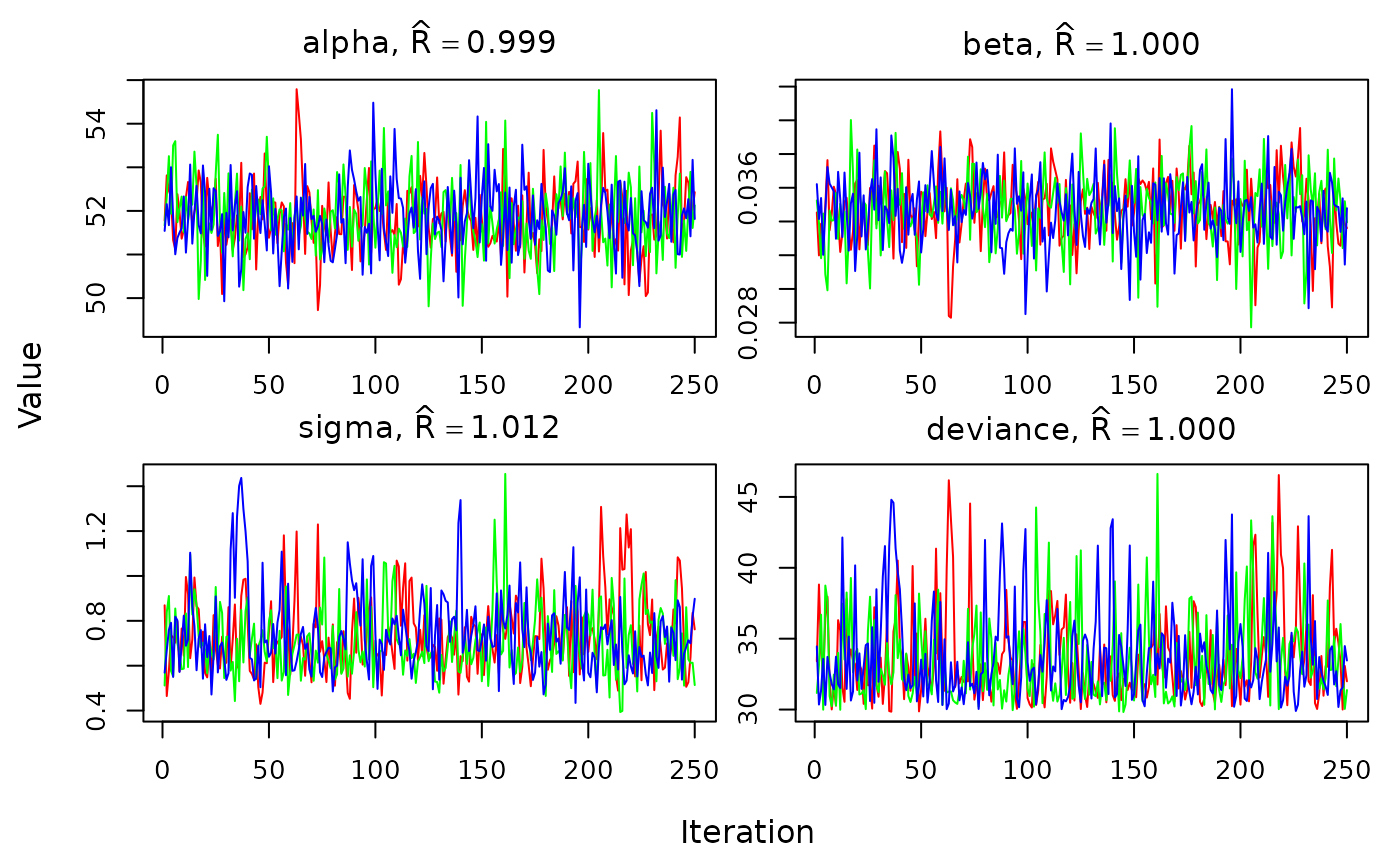
We should see the lines for each chain overlapping and not trending up or down.
Posteriors
We can quickly visualize the posterior distributions of each
parameter using the densityplot function:
densityplot(out)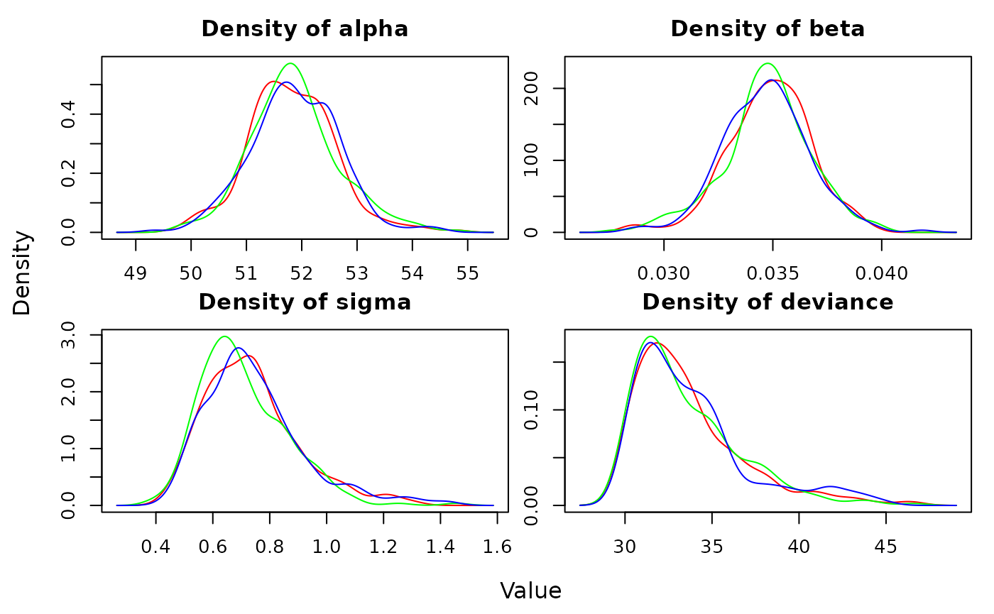
The traceplots and posteriors can be plotted together using
plot:
plot(out)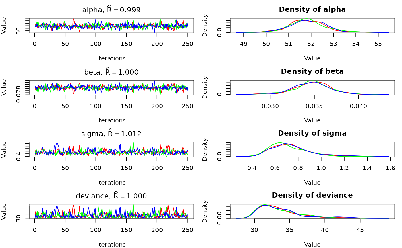
We can also generate a posterior plot manually. To do this we’ll need
to extract the actual posterior samples for a parameter. These are
contained in the sims.list element of out.
post_alpha <- out$sims.list$alpha
hist(post_alpha, xlab="Value", main = "alpha posterior")
Update
If we need more iterations or want to save different parameters, we
can use update:
# Now save mu also
params <- c(params, "mu")
out2 <- update(out, n.iter=300, parameters.to.save = params)
# Compiling model graph
#    Resolving undeclared variables
#    Allocating nodes
# Graph information:
#    Observed stochastic nodes: 16
#    Unobserved stochastic nodes: 3
#    Total graph size: 74
#
# Initializing model
#
# Adaptive phase.....
# Adaptive phase complete
#
# No burn-in specified
#
# Sampling from joint posterior, 300 iterations x 3 chains
#
#
# Calculating statistics.......
#
# Done.
The mu parameter is now in the output:
out2
# JAGS output for model '/tmp/Rtmp32mRJh/fileab4a797205d3', generated by jagsUI.
# Estimates based on 3 chains of 1300 iterations,
# adaptation = 100 iterations (sufficient),
# burn-in = 1000 iterations and thin rate = 2,
# yielding 450 total samples from the joint posterior.
# MCMC ran for 0 minutes at time 2026-01-29 15:20:59.484717.
#
#            mean    sd   2.5%    50%  97.5% overlap0 f  Rhat n.eff
# alpha    51.828 0.771 50.365 51.806 53.435    FALSE 1 1.003   450
# beta      0.035 0.002  0.031  0.035  0.038    FALSE 1 1.003   450
# sigma     0.730 0.157  0.504  0.700  1.131    FALSE 1 1.027    87
# mu[1]    59.985 0.353 59.328 59.982 60.704    FALSE 1 1.003   450
# mu[2]    60.860 0.313 60.288 60.860 61.474    FALSE 1 1.003   450
# mu[3]    60.812 0.315 60.234 60.812 61.430    FALSE 1 1.003   450
# mu[4]    61.736 0.277 61.220 61.732 62.300    FALSE 1 1.003   450
# mu[5]    63.281 0.225 62.839 63.278 63.727    FALSE 1 1.002   450
# mu[6]    63.909 0.210 63.490 63.911 64.327    FALSE 1 1.002   450
# mu[7]    64.549 0.200 64.165 64.547 64.936    FALSE 1 1.002   450
# mu[8]    64.470 0.201 64.086 64.469 64.860    FALSE 1 1.002   450
# mu[9]    65.666 0.197 65.299 65.656 66.033    FALSE 1 1.003   450
# mu[10]   66.422 0.206 66.037 66.420 66.807    FALSE 1 1.004   450
# mu[11]   67.243 0.224 66.804 67.238 67.657    FALSE 1 1.005   450
# mu[12]   67.305 0.226 66.859 67.299 67.722    FALSE 1 1.005   450
# mu[13]   68.634 0.270 68.096 68.629 69.166    FALSE 1 1.005   450
# mu[14]   69.326 0.298 68.763 69.321 69.918    FALSE 1 1.005   450
# mu[15]   69.868 0.321 69.265 69.864 70.527    FALSE 1 1.005   450
# mu[16]   71.147 0.380 70.422 71.141 71.922    FALSE 1 1.004   450
# deviance 33.533 2.941 30.202 32.717 40.939    FALSE 1 1.030    82
#
# Successful convergence based on Rhat values (all < 1.1).
# Rhat is the potential scale reduction factor (at convergence, Rhat=1).
# For each parameter, n.eff is a crude measure of effective sample size.
#
# overlap0 checks if 0 falls in the parameter's 95% credible interval.
# f is the proportion of the posterior with the same sign as the mean;
# i.e., our confidence that the parameter is positive or negative.
#
# DIC info: (pD = var(deviance)/2)
# pD = 4.2 and DIC = 37.77
# DIC is an estimate of expected predictive error (lower is better).
This is a good opportunity to show the whiskerplot
function, which plots the mean and 95% CI of parameters in the
jagsUI output:
whiskerplot(out2, 'mu')