Call JAGS from R — jags • jagsUI

The jags function is a basic user interface for running JAGS analyses via package rjags inspired by similar packages like R2WinBUGS, R2OpenBUGS, and R2jags. The user provides a model file, data, initial values (optional), and parameters to save. The function compiles the information and sends it to JAGS, then consolidates and summarizes the MCMC output in an object of class jagsUI.

jags(data, inits, parameters.to.save, model.file,
  n.chains, n.adapt=NULL, n.iter, n.burnin=0, n.thin=1,
  modules=c('glm'), factories=NULL, parallel=FALSE, 
  n.cores=NULL, DIC=TRUE, store.data=FALSE,
  codaOnly=FALSE,seed=NULL, bugs.format=FALSE, verbose=TRUE)

Arguments

data: A named list of the data objects required by the model, or a character vector containing the names of the data objects required by the model. Use of a character vector will be deprecated in the next version - switch to using named lists.
inits: A list with n.chains elements; each element of the list is itself a list of starting values for the BUGS model, or a function creating (possibly random) initial values. If inits is NULL, JAGS will generate initial values for parameters.
parameters.to.save: Character vector of the names of the parameters in the model which should be monitored.
model.file: Path to file containing the model written in BUGS code
n.chains: Number of Markov chains to run.
n.adapt: Number of iterations to run in the JAGS adaptive phase. The default is NULL, which will result in the function running groups of 100 adaptation iterations (to a max of 10,000) until JAGS reports adaptation is sufficient. If you set n.adapt manually, 1000 is the recommended minimum value.
n.iter: Total number of iterations per chain (including burn-in).
n.burnin: Number of iterations at the beginning of the chain to discard (i.e., the burn-in). Does not include the adaptive phase iterations.
n.thin: Thinning rate. Must be a positive integer.
modules: List of JAGS modules to load before analysis. By default only module 'glm' is loaded (in addition to 'basemod' and 'bugs'). To force no additional modules to load, set modules=NULL.
factories: Optional character vector of factories to enable or disable, in the format <factory> <type> <setting>. For example, to turn TemperedMix on you would provide 'mix::TemperedMix sampler TRUE' (note spaces between parts). Make sure you have the corresponding modules loaded as well.
parallel: If TRUE, run MCMC chains in parallel on multiple CPU cores
n.cores: If parallel=TRUE, specify the number of CPU cores used. Defaults to total available cores or the number of chains, whichever is smaller.
DIC: Option to report DIC and the estimated number of parameters (pD). Defaults to TRUE.
store.data: Option to store the input dataset and initial values in the output object for future use. Defaults to FALSE.
codaOnly: Optional character vector of parameter names for which you do NOT want to calculate detailed statistics. This may be helpful when you have many output parameters (e.g., predicted values) and you want to save time. For these parameters, only the mean value will be calculated but the mcmc output will still be found in $sims.list and $samples.
seed: Option to set a custom seed to initialize JAGS chains, for reproducibility. Should be an integer. This argument will be deprecated in the next version, but you can always set the outside the function yourself.
bugs.format: Option to print JAGS output in classic R2WinBUGS format. Default is FALSE.
verbose: If set to FALSE, all text output in the console will be suppressed as the function runs (including most warnings).

Details

Basic analysis steps:

Collect and package data
Write a model file in BUGS language
Set initial values
Specify parameters to monitor
Set MCMC variables and run analysis
Optionally, generate more posterior samples using the update method.

See example below.

Value

An object of class jagsUI. Notable elements in the output object include:

sims.list: A list of values sampled from the posterior distributions of each monitored parameter.
summary: A summary of various statistics calculated based on model output, in matrix form.
samples: The original output object from the rjags package, as class mcmc.list.
model: The rjags model object; this will contain multiple elements if parallel=TRUE.

Author

Ken Kellner contact@kenkellner.com.

Examples

#Analyze Longley economic data in JAGS
  
#Number employed as a function of GNP
  
######################################
##   1. Collect and Package Data    ##
######################################
  
#Load data (built into R)
  
data(longley)
head(longley)
#>      GNP.deflator     GNP Unemployed Armed.Forces Population Year Employed
#> 1947         83.0 234.289      235.6        159.0    107.608 1947   60.323
#> 1948         88.5 259.426      232.5        145.6    108.632 1948   61.122
#> 1949         88.2 258.054      368.2        161.6    109.773 1949   60.171
#> 1950         89.5 284.599      335.1        165.0    110.929 1950   61.187
#> 1951         96.2 328.975      209.9        309.9    112.075 1951   63.221
#> 1952         98.1 346.999      193.2        359.4    113.270 1952   63.639
  
#Separate data objects
  
gnp <- longley$GNP
employed <- longley$Employed
n <- length(employed)

#Input data objects must be numeric, and must be
#scalars, vectors, matrices, or arrays.
  
#Package together
data <- list(gnp=gnp,employed=employed,n=n)
    
######################################
##      2. Write model file         ##
######################################

#Write a model in the BUGS language

#Generate model file directly in R
#(could also read in existing model file)

#Identify filepath of model file
modfile <- tempfile()

#Write model to file
writeLines("
model{

  #Likelihood
  for (i in 1:n){ 

    employed[i] ~ dnorm(mu[i], tau)     
    mu[i] <- alpha + beta*gnp[i]

  }
    
  #Priors
  alpha ~ dnorm(0, 0.00001)
  beta ~ dnorm(0, 0.00001)
  sigma ~ dunif(0,1000)
  tau <- pow(sigma,-2)

}
", con=modfile)
  
######################################
##    3. Initialize Parameters      ##
######################################
  
#Best to generate initial values using function

inits <- function(){  
  list(alpha=rnorm(1,0,1),beta=rnorm(1,0,1),sigma=runif(1,0,3))  
}
  
#In many cases, JAGS can pick initial values automatically;
#you can leave argument inits=NULL to allow this.

######################################
##  4. Set parameters to monitor    ##
######################################

#Choose parameters you want to save output for
#Only parameters in this list will appear in output object
#(deviance is added automatically if DIC=TRUE)

#List must be specified as a character vector

params <- c('alpha','beta','sigma')

######################################
##        5. Run Analysis           ##
######################################

#Call jags function; specify number of chains, number of adaptive iterations,
#the length of the burn-in period, total iterations, and the thin rate.

out <- jags(data = data,
            inits = inits,
            parameters.to.save = params,
            model.file = modfile,
            n.chains = 3,
            n.adapt = 100,
            n.iter = 1000,
            n.burnin = 500,
            n.thin = 2)
#> 
#> Processing function input....... 
#> 
#> Done. 
#>  
#> Compiling model graph
#>    Resolving undeclared variables
#>    Allocating nodes
#> Graph information:
#>    Observed stochastic nodes: 16
#>    Unobserved stochastic nodes: 3
#>    Total graph size: 74
#> 
#> Initializing model
#> 
#> Adaptive phase, 100 iterations x 3 chains 
#> If no progress bar appears JAGS has decided not to adapt 
#>  
#> 
#>  Burn-in phase, 500 iterations x 3 chains 
#>  
#> 
#> Sampling from joint posterior, 500 iterations x 3 chains 
#>  
#> 
#> Calculating statistics....... 
#> 
#> Done. 

#Arguments will be passed to JAGS; you will see progress bars
#and other information

#Examine output summary

out
#> JAGS output for model '/tmp/RtmppiOn4k/file34c05db75ecf', generated by jagsUI.
#> Estimates based on 3 chains of 1000 iterations,
#> adaptation = 100 iterations (sufficient),
#> burn-in = 500 iterations and thin rate = 2,
#> yielding 750 total samples from the joint posterior. 
#> MCMC ran for 0.001 minutes at time 2024-01-30 09:20:52.060573.
#> 
#>            mean    sd   2.5%    50%  97.5% overlap0 f  Rhat n.eff
#> alpha    51.831 0.811 50.264 51.869 53.427    FALSE 1 0.998   750
#> beta      0.035 0.002  0.031  0.035  0.039    FALSE 1 1.000   750
#> sigma     0.739 0.167  0.496  0.720  1.132    FALSE 1 1.001   750
#> deviance 33.672 3.088 30.043 32.842 41.465    FALSE 1 1.002   750
#> 
#> Successful convergence based on Rhat values (all < 1.1). 
#> Rhat is the potential scale reduction factor (at convergence, Rhat=1). 
#> For each parameter, n.eff is a crude measure of effective sample size. 
#> 
#> overlap0 checks if 0 falls in the parameter's 95% credible interval.
#> f is the proportion of the posterior with the same sign as the mean;
#> i.e., our confidence that the parameter is positive or negative.
#> 
#> DIC info: (pD = var(deviance)/2) 
#> pD = 4.8 and DIC = 38.45 
#> DIC is an estimate of expected predictive error (lower is better).

#Look at output object elements
names(out)
#>  [1] "sims.list"   "mean"        "sd"          "q2.5"        "q25"        
#>  [6] "q50"         "q75"         "q97.5"       "overlap0"    "f"          
#> [11] "Rhat"        "n.eff"       "pD"          "DIC"         "summary"    
#> [16] "samples"     "modfile"     "model"       "parameters"  "mcmc.info"  
#> [21] "run.date"    "parallel"    "bugs.format" "calc.DIC"   

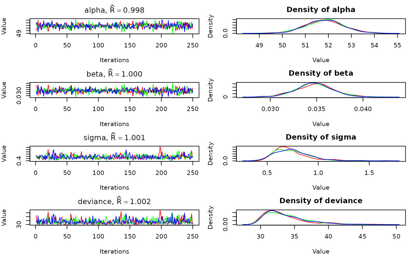
#Plot traces and posterior densities
plot(out)


#Plot traces
traceplot(out)


#Update model another 1000 iterations
out <- update(out,n.iter = 1000)
#> Compiling model graph
#>    Resolving undeclared variables
#>    Allocating nodes
#> Graph information:
#>    Observed stochastic nodes: 16
#>    Unobserved stochastic nodes: 3
#>    Total graph size: 74
#> 
#> Initializing model
#> 
#> Adaptive phase..... 
#> Adaptive phase complete 
#>  
#> No burn-in specified 
#>  
#> Sampling from joint posterior, 1000 iterations x 3 chains 
#>  
#> 
#> Calculating statistics....... 
#> 
#> Done.