ubms is an R package for fitting Bayesian hierarchical models of animal occurrence and abundance. The package has a formula-based interface compatible with unmarked, but the model is fit using MCMC with Stan instead of using maximum likelihood. Currently there are Stan versions of unmarked functions occu, occuRN, colext, occuTTD, pcount, distsamp, and multinomPois. These functions follow the stan_ prefix naming format established by rstanarm. For example, the Stan version of the unmarked function occu is stan_occu.
Advantages compared to unmarked:
- Obtain posterior distributions of parameters and derived parameters
- Include random effects in parameter formulas (same syntax as
lme4) - Assess model fit using WAIC and LOO via the loo package
Disadvantages compared to unmarked:
- MCMC is slower than maximum likelihood
- Not all model types are supported
- Potential for convergence issues
Installation
ubms is on CRAN:
install.packages("ubms")Alternatively, the latest development version can be installed from Github:
# install.packages("devtools")
devtools::install_github("kenkellner/ubms")
Example
Simulate occupancy data including a random effect on occupancy:
library(ubms)

set.seed(123)
dat_occ <- data.frame(x1=rnorm(500))
dat_p <- data.frame(x2=rnorm(500*5))

y <- matrix(NA, 500, 5)
z <- rep(NA, 500)

b <- c(0.4, -0.5, 0.3, 0.5)

re_fac <- factor(sample(letters[1:26], 500, replace=T))
dat_occ$group <- re_fac
re <- rnorm(26, 0, 1.2)
re_idx <- as.numeric(re_fac)

idx <- 1
for (i in 1:500){
  z[i] <- rbinom(1,1, plogis(b[1] + b[2]*dat_occ$x1[i] + re[re_idx[i]]))
  for (j in 1:5){
    y[i,j] <- z[i]*rbinom(1,1,
                    plogis(b[3] + b[4]*dat_p$x2[idx]))
    idx <- idx + 1
  }
}
Create unmarked frame:
umf <- unmarkedFrameOccu(y=y, siteCovs=dat_occ, obsCovs=dat_p)Fit a model with a random intercept, using 3 parallel cores:
(fm <- stan_occu(~x2 ~x1 + (1|group), umf, chains=3, cores=3, seed=123))##
## Call:
## stan_occu(formula = ~x2 ~ x1 + (1 | group), data = umf, chains = 3,
## cores = 3, refresh = 0, seed = 123)
##
## Occupancy (logit-scale):
## Estimate SD 2.5% 97.5% n_eff Rhat
## (Intercept) 0.335 0.283 -0.205 0.911 977 1.003
## x1 -0.458 0.120 -0.698 -0.221 4080 0.999
## sigma [1|group] 1.335 0.254 0.915 1.908 2005 1.000
##
## Detection (logit-scale):
## Estimate SD 2.5% 97.5% n_eff Rhat
## (Intercept) 0.382 0.0602 0.266 0.501 4273 1
## x2 0.586 0.0630 0.465 0.712 5152 1
##
## LOOIC: 2268.202
## Runtime: 31.974 secExamine residuals for occupancy and detection submodels (following Wright et al. 2019). Each panel represents a draw from the posterior distribution.
plot(fm)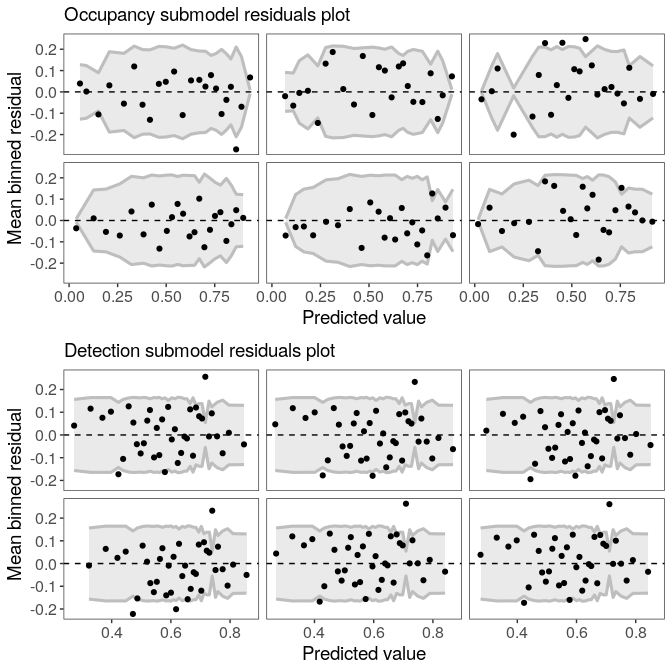
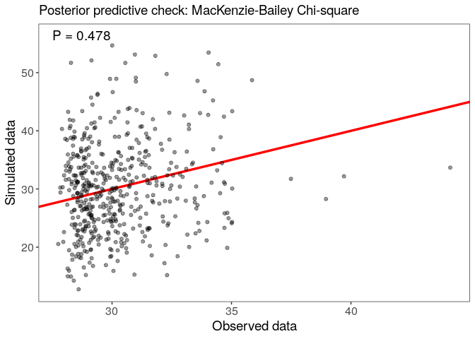
Assess model goodness-of-fit with a posterior predictive check, using the MacKenzie-Bailey chi-square test:
Look at the marginal effect of x2 on detection:
plot_effects(fm, "det")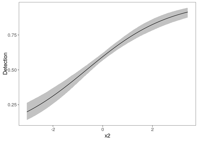
A more detailed vignette for the package is available here.